
Neo4J is still the first name you think of when uttering the phrase “graph database” and ArangoDB in my opinion is rising rapidly to take the lead. It pains me to say it as I’ve put considerable hours into Neo4J, but there we have it. There are some whitepapers and comparison sites that level peg them, but using the same logic, a Ferrari and a Cirrus aircraft can both give you a comfortable journey down a runway at 150mph, but only the Cirrus can soar through the skies. Arango is the Cirrus.
ArangoDB is something I’ve been aware of for a while thanks to Phil Shafer and Jeremy Schulman (circa 2018?), but I’ve not really had the need to dig deep because Neo4J has satisfied my needs up until recently. The event which caused me to dig deeper was akin to Apache2 and GPLv3 going together like my love for Marmite. This last twelve months, I’ve also had major interest in AWS DynamoDB and have found NoSQL to be fantastic, if you apply some discipline to single table design and some common sense to developing data access patterns.
Here’s what you need to know if you can’t be bothered to read the rest:
ArangoDB
- Apache2 for open-source use
- Offers NoSQL capabilities and groups documents together into logical entities called collections
- Can link collections together via edges, which form named graphs and anonymous graph structures
- Works with native JSON
- The query language AQL (ArangoDB Query Language) is simple and mighty powerful
- Go native drivers (absolute win)
- Very friendly team (like seriously)
Below, I scratch the surface on ArangoDB, leaning heavily on their training material and docs.
- Udemy course: https://arangodb.com/udemy
- 14 day free Oasis ArangoDB cloud instance
- Free graph course for beginners
If you wanted to run this on Docker, here’s how to get going super-fast. Note, no authentication is set here so please don’t run this in production. It’s for testing and kicking the tyres.
docker run -e ARANGO_NO_AUTH=1 -p 8529:8529 -d arangodb
If you want persistent data between Docker restarts try this, changing the directory name arangodbtest appropriately.
docker run -e ARANGO_NO_AUTH=1 -p 8529:8529 -v /home/$USER/arangodbtest:/var/lib/arangodb3-d arangodb
The training material is based on two files, called flights.json and airports.json. They are available from this blog by clicking the links as well as the ArangoDB website. You can load them into ArangoDB by creating a collection for airports as a standard document collection and by creating a collection for flights as an edge collection. When you’ve created each collection, you can go to the collection settings and upload the JSON files to them like below. Note, I created a database called test for this.

Go make a coffee and come back when importing the flights data. It’s 95MB in size and take some time to import.
A quick tour on collections
Some questions arose early days in my mind as I started to compare it against DynamoDB. Could I have documents in a collection with some field variances? For instance, could I have these records in a collection?
// The nerd collection
[
  {"name": "bob", "hasacar": true },
  {"name": "alice", "hasabike": true }
]
The answer is of course yes. Here’s an AQL query to retrieve the data I’m interested in.
FOR doc in test
    RETURN {name: doc.name, car: doc.hasacar, bike: doc.hasabike}
And the projected data from the query.
| Name | Has a car | Has a bike |
|---|---|---|
| bob | true | null |
| alice | null | true |
Outliers are always present when modelling things and it’s important therefore we have some flexibility in the tools we use for modelling and querying them. Regarding the above, integrity checks will require conditionals to detect the presence of odd fields that vary in their presence before using them in loop or aggregate based queries. The important thing is, I can include additional information when required, without having change a schema. ArangoDB is therefore schemaless just like Neo4J. The mental thorn that sprang the question was the ability to group similar documents in a collection. So what is similar? Well, it’s whatever you decide. In networking, I might assign a group of leaf switches in a given data hall to a collection. They might have different model numbers and different attributes altogether. Some might have uplink ports, some might not at all.
One of the things I come across regularly, is ordered state held in JSON. An example would be firewall rules on Junos. The order of them absolutely matters and in projects, I’ve gone to great lengths, like encoding data into TLVs with mechanisms to ensure the integrity and order of this data remains intact between ETL operations.
Thankfully, ArangoDB holds true to ordered state between load and extractions! Here’s an example of ordered data in a document in a collection. Naturally, this doesn’t apply if you sort the data and explicitly change the order.
// Document addition for Walter
{
  "name": "walter",
  "wards": [
    "bob",
    "alice"
  ]
}
| Name | Has a car | Has a bike | Wards |
|---|---|---|---|
| bob | true | null | null |
| alice | null | true | null |
| walter | null | null | [“bob”,“alice”] |
If you export the data from ArangoDB, the array order is maintained. It might seem simple but making assumptions that “it will probably be ok” is outright foolish when you rely upon specific behaviour. I’ve tried different data sets and order is maintained.
CRUD Hello-World
Below are helpers for CRUD operations on ArangoDB.
Arango uses some reserved field names. It’s common to set the _key field but it’s good to be aware of how ArangoDB operates.
_key_id_rev_from// for edge collection documents_to// for edge collection documents
Document fields have to be unique, a string, of no more than 254 bytes and can contain these characters: _-:.@()+,=;$!*'%
Create (Insert)
Creating is quite simple!
INSERT {_key: "Test"} INTO 'airports' RETURN NEW

// This also works, note NEW has to be capitalised. Probably easier to keep the ArrangoDB keywords capitalised.
insert { _key: "Test" } into airports return NEW
Read (Document)
These all do the same thing, which is read from the collection.
RETURN DOCUMENTS("airports/Test")
RETURN DOCUMENTS("airports", ['Test'])
If you want to return entire docs, you can do things like project the data set you require. I touched on this earlier.
FOR doc in "airports"
    RETURN {name: doc._id, doc.name }
Update (Update)
Updates are simple. This update adds the field name with value Bob to the airports collection document with field “Test”.
UPDATE {_key: "Test" } WITH {name: "Bob" } IN airports
RETURN NEW
You can use the For Loop construct here to do multiple updates.
FOR doc IN ["Test"]
  UPDATE doc WITH {colour: "red" } IN airports
  RETURN NEW
Delete (Remove)
Let’s remove a document from a collection. You can use a for loop too here. Remove is a single query, in a collection executed in a single operation.
FOR docs in ["Test"]
  REMOVE docs IN airports
Filtering
We might want to query and filter on specific fields. Here is an example of trying to find data on a plane’s tail number.
Filter statements must evaluate to true or false and support logical operators: AND/&&, OR/||, NOT/!
FOR flight in flights
  FILTER flight.TailNum == "N592ML"
  RETURN flight
Indexes
ArangoDB has default indexes on _key in a collection and on _from and _to on an edge collection.
There are numerous types of index available for you to create and on pay attention to the database engine being used.
The persistent index is actually what they refer to as the Hash index when running on RocksDB.
Adding an Index can speed things up a lot. For the tailnumber example in the training material, the speed up was noticeable. Without the index the query took ~500mS and with a persistent index (Hash) based on the TailNumber field, the query ran at ~2.4mS, which is an incredible gain, given there are some 280,000+ records. I love the aspect of their training because they made it fun but also tangible, beyond a hello world.
GeoJSON
ArangoDB out of the box supports GeoJSON which is based on Google’s S2 computation spherical geometry system. What this means is, we can query on geospatial data and build things like map views. GeoJSON is implemented as a set of Geo functions that are natively available to AQL. I swore out loud when I saw this the first time. It’s just neat. OpenStreetMap visualisations are also built in.
First, let’s make sure the records are there and checkout what the longitude and latitude fields are called in the record.
FOR airport in airports
  FILTER airport.state == "TX"
  RETURN airport
Now we know that the records are .long and .lat, here’s the query that generates a map view.
FOR airport in airports
  FILTER airport.state == "TX"
  RETURN GEO_POINT(airport.long, airport.lat)
The GEO_POINT function actually takes the long and lat inputs and returns a Geo spatial point object which looks like below:
{
  "type": "Point",
  "coordinates": {
    coordinateNumber,
    coordinateNumber
  }
}
Where this comes in to its own, is searching for proximity. The training material queries look for airports that are within close proximity, but for your use case it, it could be a milk supplier or MacDonalds. This is very useful indeed!
FOR airport in airports
  FILTER GEO_DISTANCE([-95.01792778, 30.68586111], [airport.long, airport.lat]) <= 50000
  RETURN airport
This query shows airports within a 50km radius of the long/lat coordinates in the first argument to GEO_DISTANCE and generates a map showing the points. How cool is this?
FOR airport in airports
  FILTER GEO_DISTANCE([-95.01792778, 30.68586111], [airport.long, airport.lat]) <= 50000
  RETURN GEO_POINT(airport.long, airport.lat)
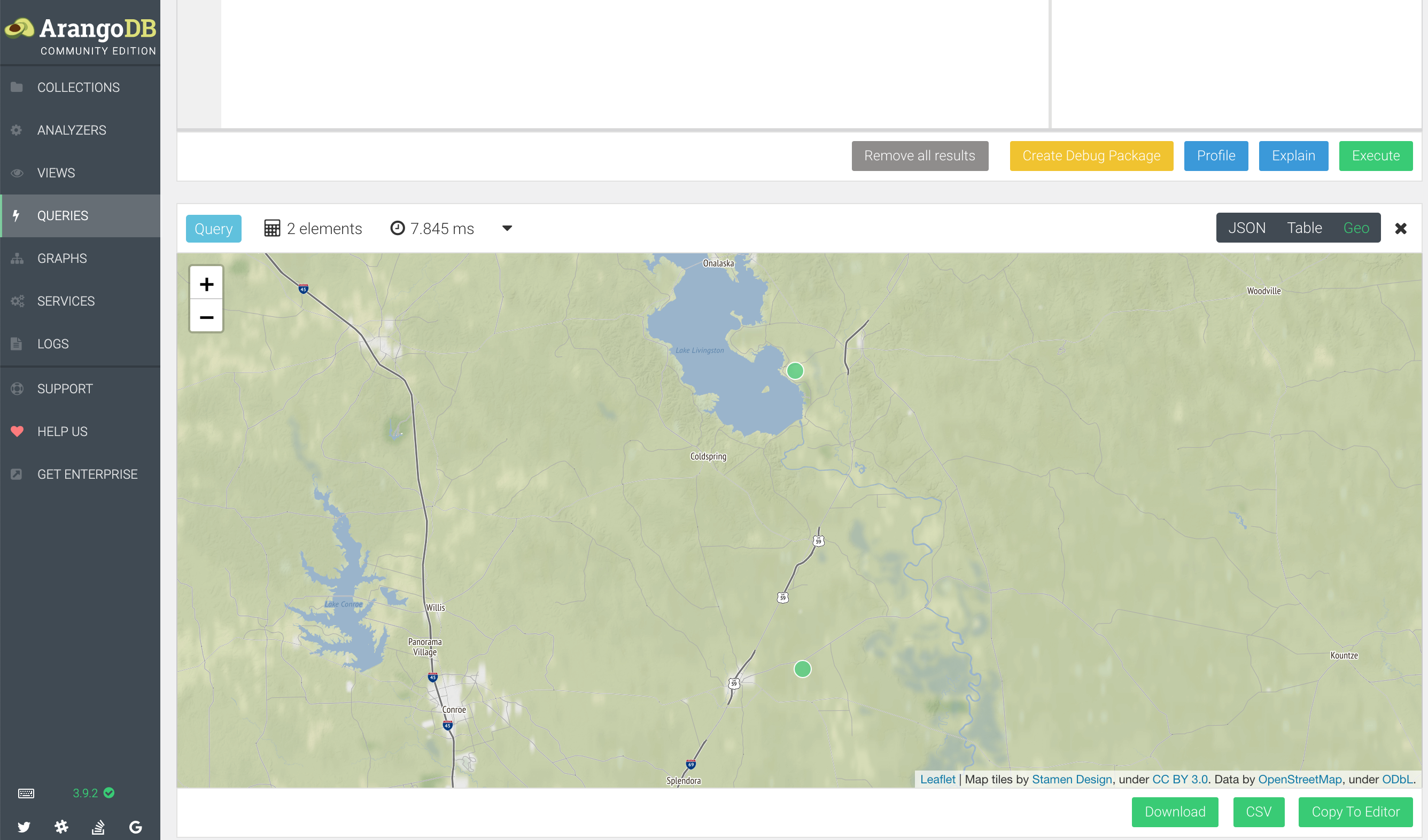
This made me very, very excited.
Joins, Collect & Aggregate
You can join collections through nested for loops.
For instance, we can query through the airports in Dallas and the find what flights are heading to that airport.
FOR airport in airports
  FILTER airport.city == "Dallas"
  FOR flight in flights
    FILTER flight._to == airport._id
    RETURN {
      "airport": airport.name,
      "flight": flight.FlightNum
    }
The issue with some joins, especially in multi-cluster environments is the task duration can rocket up, especially when network hops are considered. You can embed data into JSON documents to help with this or collect data. Thinking about data locality will help speed up complex arrangements too.
Here, we use collect in a manner which is analogous to: Define what is being collected and assign it to the variable.
FOR airport in airports
  COLLECT state = airport.state WITH COUNT INTO total
  RETURN {
    State: state,
    "Total airports": total
  }
You can also sort the responses. The output defaults to ascending if the keyword desc isn’t included.
FOR airport in airports
  COLLECT state = airport.state WITH COUNT INTO total
  SORT total desc
  RETURN {
    State: state,
    "Total airports": total
  }
For aggregations, we can find the longest flight distance and shortest distance. Aggregate is always a clause of the collect keyword and be done post collect as well as with collect, using different AQL constructs.
FOR flight in flights
  COLLECT AGGREGATE
  minDistance = MIN(flight.Distance),
  maxDistance = MAX(flight.Distance),

  RETURN {
    "Shortest flight": minDistance,
    "Longest flight": maxDistnace
  }
The magic here is that AGGREGATE means we don’t have to iterate using multiple for loops. Aggregate has quite a few functions including:
- MIN
- MAX
- SUM
- AVERAGE
- VARIANCE_POPULATION
- VARIANCE_SAMPLE
- STDDEV_POPULATION
- STDDEV_SAMPLE
- UNIQUE
- SOTED_UNIQUE
- COUNT_UNIQUE
There are lots of references in the AQL documentation like “This is how you would do it with SQL”. It’s quite handy in order to get your head around how some of this works.
Graphs!
Now we hit the good stuff.
Graphs in ArangoDB are achieved through linking standard document collections and edge collections. The collection documents are the vertices, and the edge collection documents are the edges. By connecting these collections, it’s easy to form graph relationships from similarly formed objects. These edge collections have fields _to and _from which define the relationship. The documents in those collection are identical other than the additional fields to normal collections, meaning you can add arbitrary data to them.
Now, you might be wondering if this is noteworthy, and it is. Imagine that you’re modelling an IP Fabric (Clos fabric) with Arango. You can treat nodes separately from their connecting interfaces and so modelling becomes flexible. With Neo4J, you would need to manipulate each node’s properties or even worse, prune it from the graph through Cypher statements. Modelled in this way, each data center could have a collection of spines, leafs and interconnects defined as separate docs. It provides horizontal scalability and logical data grouping that is easily traversable. Neo4J doesn’t have this capability and requires you do a set of queries to narrow down your scope. ArangoDB out of the box solves this beautifully. There are two types of graph in ArangoDB, named graphs and anonymous graphs.
Named Graphs
- Managed by ArangoDB
- Transactional Modifications
- Edge Consistency
- Edge Clean-Up
- Graph Module (arangosh, drivers)
- AQL support
Anonymous Graphs
Also referred to as loosely coupled collection sets.
- Integrity checks done client side
- Readability improved?
- AQL support
Graph Syntax
FOR
  vertexVariableName,
  edgeVariableName,
  pathVariableName,
  IN
  traversalExpression
  directionExpression
- vertextVariableName = the current vertex in traversal, the only required option
- edgeVariableName = optional: the current edge in traversal, the special edge collection with
_toand_fromfields - pathVariableName = optional: contains two arrays, first is all vertices of the path, second is all edges of the path
- traversalExpression = IN min..maxs
- directionExpression = INBOUND or OUTBOUND or ANY
Start vertex form:
- ID String, declares the quoted collection and document ID
- Document, useful for more complex queries
FOR v, e, p IN 1..1 OUTBOUND
  'airports/JFK'
  GRAPH 'flights'
  RETURN p
You can also use a list of edge collections instead of the GRAPH reference, which would mean it’s an anonymous graph.
Writing filters for Graph queries can be fun.
Filters can have multiple statements, or you can write multiple filter statements. Below the traversal length is set to min 1 and max 1, meaning direct flights in this example.
FOR airport in airports
  FILTER airport.city == "San Francisco" && airport.vip == true
  FOR v, e, p IN 1..1 OUTBOUND
  airport flights
  FILTER v._id == 'airports/KOA'
  RETURN p
Fundamentally the same as the below. This syntax is the hardest bit I’ve come across so far, but once you spend five minutes reading the docs, it becomes grokkable.
FOR v, e, p IN 1..1 OUTBOUND 'airports/SFO'
GRAPH 'flights'
FILTER v._id == 'airports/KOA'
RETURN p
Now, assuming the searching user wants some cheaper flights, you can do something like this:
FOR airport in airports
  FILTER airport.city == "San Francisco" && airport.vip == true
  FOR v, e, p IN 2..3 OUTBOUND
  airport flights
  FILTER v._id == "airports/KOA"
  FILTER p.edges[*].Month ALL == 1
  FILTER p.edges[*].Day ALL == 3
  LIMIT 10
  RETURN p
There’s a ton of stuff to unpack. The main thing is, we ask for flights with the minimum of two hops with a max of three hops. We’ve also limited the day and month that these flights can depart.
The issue with this search as well is it doesn’t allow for connections! The next flight could be in the air by the time the current one touches down. Yikes. What is this, CDG? This set of additional filters allows for three edge connections.
FOR airport in airports
  FILTER airport.city == "San Francisco" && airport.vip == true
  FOR v, e, p IN 2..3 OUTBOUND
  airport flights
  FILTER v._id == "airports/KOA"
  FILTER p.edges[*].Month ALL == 1
  FILTER p.edges[*].Day ALL == 3
  FILTER DATE_ADD(p.edges[0].ArrTimeUTC, 20, 'minutes') < p.edges[1].DepTimeUTC
  FILTER DATE_ADD(p.edges[1].ArrTimeUTC, 20, 'minutes') < p.edges[2].DepTimeUTC
  LIMIT 10
  RETURN p
These queries are incredibly powerful and remind me of the kind of data filtering I do on user interfaces with JavaScript. Which leads me to…
Foxx Microservices
Urgh. I hear you, yet another microservice thing. But hold up! This is actually quite useful and cool, so read on (despite the random name Foxx sticking out like a sore thumb). Foxx isn’t about how to scale-up or scale-out the ArangoDB, but how you can embed some of your query and business logic into custom REST API endpoints through Swagger (OpenAPI), all through a few simple lines of JavaScript. Other databases might call these stored procedures, but the difference with ArangoDB is, they’ve available via a user defined custom REST endpoint. For the security minded, yes, there are options available for authentication plus many other things you might want to wrap your REST endpoint in. It’s JavaScript after all.
This reminds me of the SDN controller era of networking like the HP VAN controller and OpenDayLight. With the SDN controllers, you would build a package and load it to the controller as a capability. The concept of baking a small application and loading it onto the database itself is really nice. This is the same, but for the database and your embodied logic has no requirement of using the database as a document store, graph or even using the database at all. I wonder how many people have gone “Huh, it’s a convenient place to put some helper functions”. In my mind’s eye, it’s like an SDN controller without any south-bound interface to programmable network devices and very handy as an arbitrary core engine to an application, especially so if you run it on Docker!
Information on Foxx: https://www.arangodb.com/docs/stable/foxx.html
Wrap-Up
For NoSQL and for graph, ArangoDB is really quite impressive. I’m actively using it for modelling brownfield network scenarios and will be exploring the Go aspects too. If you’re curious, it’s absolutely worth taking the free course and you can make your own mind up. Neo4J will forever have a special place in my heart, but ArangoDB has taken the lead.